Modern portfolio theory is based on the use of statistical and mathematical methods. Its distinguishing feature is the relationship between market risk and return, namely: an investor must build a relatively risky portfolio in order to expect a relatively high return. Using this approach requires certain computer and mathematical support. In many cases, a combination of the above approaches will be strategically correct.

Today, the two most common models for determining portfolio characteristics are the Markowitz model and the Sharpe model. Both models were created and work successfully in the already established relatively stable Western stock markets. Unfortunately, the Ukrainian stock market cannot yet be called stable. Therefore, an attempt was made to create a model capable of successfully functioning in the conditions of an emerging, developing and reorganizing stock market, which is what the stock market of Ukraine is today. The proposed model was called “Quasi-Sharpe” (due to its similarity in general terms with the Sharpe model) and will be presented below.

Markowitz model

In 1952, Harry Markowitz published a seminal work that is the basis for the approach to investment from the point of view of modern portfolio theory. The Markowitz approach begins with the assumption that the investor currently has a specific amount of money to invest. This money will be invested for a certain period of time, called the holding period. At the end of the holding period, the investor sells the securities that were purchased at the beginning of the period, after which he either uses the resulting income for consumption or reinvests the income in various securities (or does both at the same time).

Markowitz's approach to decision making makes it possible to adequately take into account both of these goals. A consequence of the presence of two conflicting goals is the need to diversify by purchasing not one, but several securities.

The model is based on the fact that the profitability indicators of various securities are interconnected: with an increase in the profitability of some securities, there is a simultaneous increase in other securities, others remain unchanged, and for others, on the contrary, the profitability decreases. This type of dependence is not deterministic, i.e. uniquely determined, but stochastic and is called correlation.

It is rational to use the Markowitz model in a stable state of the stock market, when it is desirable to form a portfolio of securities of a different nature belonging to different industries. The main drawback of the Markowitz model is that the expected return on securities is assumed to be equal to the average return based on historical data. Therefore, it is rational to use the Markowitz model in a stable state of the stock market, when it is desirable to form a portfolio of securities of a different nature that have a more or less long life on the stock market

Sharpe model

The Sharpe model examines the relationship between the return of each security and the return of the market as a whole. The main idea of ​​the model is that the investor does not accept risk and is ready to take it only if it involves additional benefit, i.e. an increased rate of return on invested capital compared to a risk-free investment. The risk-free rate is the rate of return on long-term government bonds with a maturity date of typically 10 to 20 years. The Sharpe model is mainly applicable when considering a large number of securities that cover a large part of the stock market. The main drawback of the model is the need to predict stock market returns and the risk-free rate of return. This model does not take into account the risk of fluctuations in risk-free returns. In addition, if the relationship between the risk-free return and the stock market return changes significantly, the model becomes distorted.

Quasi-Sharp model

The Markowitz and Sharp models were created and work successfully in Western stock markets, which are stable and relatively predictable. In countries with economies in transition, stock markets are at the stage of formation and development. There is constant reorganization going on. The Ukrainian stock market is no exception. In such conditions, the use of the Markowitz and Sharpe models leads to distortions associated with the instability of securities quotes and the stock market as a whole.

The Sharpe model examines the relationship between the return of each security and the return of the market as a whole.

Basic assumptions of the Sharpe model:

As profitability security is accepted mathematical expectation of profitability;

There is a certain risk-free rate of return, i.e., the yield of a certain security, the risk of which Always minimal compared to other securities;

Relationship deviations return of a security from the risk-free rate of return(Further: security yield deviation) With deviations profitability of the market as a whole from the risk-free rate of return(Further: market return deviation) is described linear regression function ;

Security risk means degree of dependence changes in the yield of a security from changes in the yield of the market as a whole;

It is believed that the data past periods used in calculating profitability and risk fully reflect future profitability values.

According to the Sharpe model, deviations in security returns are associated with deviations in market returns using a linear regression function of the form:

where is the deviation of the security's yield from the risk-free one;

Deviation of market returns from risk-free ones;

Regression coefficients.

Based on this formula, it is possible, based on the predicted profitability of the securities market as a whole, to calculate the profitability of any security that constitutes it:

where , are regression coefficients characterizing this security.

Theoretically, if the securities market is in equilibrium, then the coefficient will be zero. But since in practice the market is always unbalanced, it shows excess return of a given security (positive or negative), i.e. the extent to which a given security is overvalued or undervalued by investors.

The coefficient is called -risk, because it characterizes the degree of dependence of deviations in the profitability of a security from deviations in the profitability of the market as a whole. The main advantage of the Sharpe model is that the interdependence of profitability and risk is mathematically substantiated: the greater the risk, the higher the profitability of the security.

In addition, the Sharpe model has a peculiarity: there is a danger that the estimated deviation of the security's return will not belong to the constructed regression line. This risk is called residual risk. Residual risk characterizes the degree of dispersion of the deviation values ​​of a security's return relative to the regression line. Residual risk is defined as the standard deviation of the empirical points of a security's return from the regression line. The residual risk of the i-th security is denoted by .

In other words, the risk indicator of investing in a given security is determined by risk and residual risk.

In accordance with the Sharpe model, the return on a securities portfolio is the weighted average of the return indicators of the securities and its components, taking into account risk. The portfolio return is determined by the formula:

where is the risk-free return;

Expected profitability of the market as a whole;

The risk of a securities portfolio can be found by estimating the standard deviation of the function and is determined by the formula:

,

where is the standard deviation of the profitability of the market as a whole, i.e., an indicator of the risk of the market as a whole;

Risk and residual risk of the i -th security;

Using the Sharpe model to calculate portfolio characteristics, the direct problem takes the form:

The inverse problem looks similar:

In the practical application of the Sharpe model to optimize the stock portfolio, the following assumptions and formulas are used.

1). Usually, the yield on government securities, for example, domestic government loan bonds, is taken as the risk-free rate of return.

2). Expert estimates of market returns from analytical companies, the media, etc. are used as the profitability of the securities market as a whole in period t. In conditions of a developed stock market, it is customary to use any stock indices for these purposes. For a stock market that is not very large in terms of the number of securities, the average return on the securities making up the market for the same period t is taken:

where is the return on the securities market in period t;

The initial data for the calculation (the yield of securities) remains unchanged (see Table 4.9.1). In addition, the Sharpe model uses the return of the market as a whole and the risk-free return. The profitability of the market as a whole was taken on the basis of expert estimates, due to the lack of data from external sources. The weekly yield of three-month government short-term bonds was taken as the risk-free yield. Data on the profitability of the market as a whole and on risk-free profitability are presented in table. 4.9.5.

Let's consider the practical aspects of constructing a capital asset valuation model CAPM using Excel for domestic shares of OAO Gazprom.

Capital Asset Valuation Model(English)CapitalAssetsPriceModel,CAPM)– a model for assessing (forecasting) the future return of an asset for investors. The asset valuation approach was theoretically developed back in the 50s by G. Markowitz, and finally formed in the form of a model in the 60s by W. Sharp (1964), J. Trainor (1962), J. Lintner (1965), J. Mosin (1966).

The CAPM model is based on the efficient capital market hypothesis ( EfficientMarketHypothesis, EMH), created at the beginning of the 20th century by L. Bachelier and actively promoted by Y. Fama in the 60s. This hypothesis has a number of conditions regarding the method of information dissemination and the action of investors in an efficient capital market:

• Information is freely distributed and available to all investors; the market is perfectly competitive. In other words, there are no insiders who have a great advantage in making decisions and receiving excess returns (above the market average).
• Any change in information about a company immediately leads to a change in the value of its assets (shares). This eliminates the possibility of using any active investment strategy to obtain excess profits. This premise excludes the possibility of arbitrage transactions when the investor has useful information in advance, while the price of the company's assets has not yet changed.
• Investors in an efficient market have a long-term investment horizon. This eliminates the occurrence of sudden changes in asset (stock) prices and crises.
• Assets are highly liquid and absolutely divisible.

Based on the efficient market hypothesis, W. Sharp made the assumption that only market (systemic) risks will influence future stock returns. In other words, the future performance of a stock will be determined by the overall market sentiment. That’s why, by the way, he was a supporter of passive investing, when the investment portfolio is not revised due to receiving new information. It should be noted that in an efficient market it is impossible to make excess profits. This makes any active management of investments (investment portfolio) inappropriate and calls into question the effectiveness of investing in mutual funds. As a result, W. Sharpe’s model has only one factor – market risk (beta coefficient). Analyzing these postulates of an efficient market, one can notice that in the modern economy many of them are not fulfilled. The CAPM model is largely a theoretical model and can be used in practice in general.

CAPM model. Calculation formula

The formula for estimating the future return of an asset (share) using the CAPM model has the following analytical form:

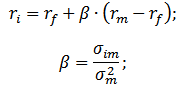
r – expected return on the asset (shares);

r f – return on a risk-free asset;

r m – average market return;

β is the beta coefficient (a measure of market risk), which reflects the sensitivity of changes in asset prices depending on market returns. This ratio is sometimes called the Sharpe ratio.

The model is a linear regression equation and shows a linear relationship between return (r) and market risk (β);

σ im is the standard deviation of the change in stock returns from the change in market returns;

σ 2 m – dispersion of market returns.

In order to better understand the CAPM model, let’s analyze it using a real example of shares of the Gazprom OJSC enterprise. To do this, we will use Excel. You can get stock quotes on the website finam.ru in the “About the Market” → “Data Export” section.

In our formula, we will take changes in the RTS index (RTSI) as market returns; it can also be the MICEX index (MICECX). For American stocks, changes in the S&P500 index are often used. Daily stock and index quotes were taken for 1 year (250 data), starting from 01/31/2014 to 01/30/2015.
Next, you need to calculate the returns of the stock (E) and index (D), using the formulas:

I would like to note that to estimate yields, the calculation formula through the natural logarithm could also be used:

The final result of calculating profitability is the same.

Calculating Beta Using Excel Formulas

To calculate the beta coefficient, you can use the INDEX and LINEST formulas, the first allows you to take the index b from the linear regression formula between the returns of the stock and the index, which corresponds to the beta coefficient. The calculation formula will be as follows:

INDEX(LINEST(E7:E256,D7:D256),1)

Calculating beta using the Regression add-on

The second option for calculating the market risk of a model is to use the add-in in the “Main Menu” → “Data” → “Data Analysis” → “Regression” section.

In the window that opens, you need to fill in two fields: “Input interval Y” and “Input interval X” with the returns of the index and stock, respectively.

The main parameters of the linear regression model will appear on a new Excel sheet. Cell B18 will display the calculated linear regression coefficient - the beta coefficient. Let's consider other obtained analysis parameters. Thus, the Multiple R (correlation coefficient) indicator between the return of a stock and the index is 0.29, which shows the low degree of dependence of the return of the stock on the return of the index. The R-squared coefficient (coefficient of determinism) reflects the accuracy of the resulting model. The accuracy is 0.08, which is very low to make adequate decisions about predicting future returns based on the relationship only with the level of market risk.

What does the beta coefficient show in the CAPM model?

The beta coefficient shows the sensitivity of changes in stock returns and market returns. In other words, it reflects the riskiness of investing in a particular asset. Beta is a measure of market risk. The sign in front of the indicator reflects their unidirectional or multidirectional movement. Let's take a closer look at the beta value in the table below:

Beta value

The Sharpe model examines the relationship between the return of each security and the return of the market as a whole.

Basic assumptions of the Sharpe model:

As profitability security is accepted mathematical expectation of profitability;

There is a certain risk-free rate of return, i.e., the yield of a certain security, the risk of which Always minimal compared to other securities;

Relationship deviations return of a security from the risk-free rate of return(Further: security yield deviation) With deviations profitability of the market as a whole from the risk-free rate of return(Further: market return deviation) is described linear regression function ;

Security risk means degree of dependence changes in the yield of a security from changes in the yield of the market as a whole;

It is believed that the data past periods used in calculating profitability and risk fully reflect future profitability values.

According to the Sharpe model, deviations in security returns are associated with deviations in market returns using a linear regression function of the form:

where is the deviation of the security's yield from the risk-free one;

Deviation of market returns from risk-free ones;

Regression coefficients.

The main drawback of the model is the need to predict stock market returns and the risk-free rate of return. The model does not take into account fluctuations in risk-free returns. In addition, if the relationship between the risk-free return and the stock market return changes significantly, the model becomes distorted. Thus, the Sharpe model is applicable when considering a large number of securities that describe b O most of the relatively stable stock market.

41.Market risk premium and beta coefficient.

Market risk premium- the difference between the expected return of the market portfolio and the risk-free rate.

Beta coefficient(beta factor) - indicator calculated for securities or a portfolio of securities. Is a measure market risk, reflecting variability profitability security (portfolio) in relation to the portfolio return ( market) on average (average market portfolio). For companies that do not have publicly traded shares, a beta can be calculated based on a comparison with the performance of peer companies. Analogues are taken from the same industry, whose business is as similar as possible to the business of a non-public company. When calculating, it is necessary to make a number of adjustments, in particular, for the difference in the capital structure of the companies being compared (debt to equity ratio).

Beta coefficient for an asset in a securities portfolio, or an asset (portfolio) relative to the market is a relation covariances of the quantities under consideration to variances reference portfolio or market, respectively :

where is the estimated value for which the Beta coefficient is calculated: the return on the asset or portfolio being evaluated, - the reference value with which the comparison is made: the return on the securities portfolio or market, - covariance estimated and reference value, - dispersion reference value.

Beta coefficient is a unit of measurement that gives a quantitative relationship between the movement of the price of a given stock and the movement of the stock market as a whole. Not to be confused with variability.

Beta coefficient is an indicator of the degree of risk in relation to an investment portfolio or specific securities; reflects the degree of stability of the price of these shares in comparison with the rest of the stock market; establishes a quantitative relationship between fluctuations in the price of a given stock and the dynamics of market prices as a whole. If this ratio is greater than 1, then the stock is unstable; with a beta coefficient less than 1 – more stable; This is why conservative investors are primarily interested in this ratio and prefer stocks with a low level.

test

2.2 Sharpe model

investment portfolio model management

The Sharpe model is based on the interdependence of the profitability of each security with the profitability of the market as a whole.

Such a model for constructing an investment portfolio as the W. Sharp model works well during periods of stable growth of the national economy.

This remark, as a rule, applies to foreign stock markets, which are characterized by more monotonous development dynamics. Using the Sharpe model for emerging markets, including stock markets such as the Russian Federation and other CIS countries, can lead to unpredictable portfolio losses and model errors. First of all, this is due to the dynamics and features of the development of these markets: they are characterized by impulsive profitability and instability, the strong influence of internal information, the dominant influence of raw materials industries on the overall dynamics of development, and the imperfection of the regulatory framework.

Main hypotheses:

· the mathematical expectation of profitability is taken as profitability;

· there is a risk-free rate of return - this is the profitability of some investment, the risk of which is always minimal in relation to other investment risks;

· the relationship between deviations of a security's yield from the risk-free rate of return and deviations of the profitability of the market as a whole from the risk-free rate of return is taken in the form of linear regression;

· the risk of a security is the dependence of changes in the profitability of a security on changes in the profitability of the market as a whole;

· estimated future profitability values ​​depend on historical data.

According to the Sharpe model, a linear regression function relates deviations in market returns to deviations in security returns of the form:

Deviation of the yield of a security from the risk-free one,

Deviation of market returns from risk-free,

b, c - regression coefficients.

Regression coefficients of the th security.

The coefficient bi is equal to zero provided that the securities market is in equilibrium.

To find portfolio characteristics using the Sharpe model, the direct problem has the form:

The inverse problem takes on a similar form:

In order to practically apply the Sharpe model for portfolio optimization purposes, the following formulas and assumptions are used.

As a rule, the risk-free rate of return is determined as the yield on government securities, an example being domestic government loan bonds.

To determine the profitability for the period of the securities market as a whole, expert estimates of market returns from the media, from analytical companies, etc. are used. Also, in a developed stock market environment, it is customary to use various stock indices to achieve these goals. For a stock market with not a very large number of securities, the average return of the securities that make up the market for the same period is taken:

Returns on the securities market during the period;

Yield of the th security for the period.

The indicator (“beta”) is a characteristic of the degree of risk of a security and shows how many times the change in the price of a security exceeds the change in the market as a whole. If beta takes a value greater than one, then this security can be classified as an instrument with an increased level of risk, this is due to the fact that its price on average moves faster than the market. A beta value less than one indicates that the risk level of this security is relatively low, because during the settlement depth period, its price changed more slowly compared to the market. If the beta is less than zero, this means that on average the movement of this security during the period of depth of calculation was opposite to the movement of the market.

Security risk is calculated using the formula:

Risk of the security;

Risk-free return during the period;

The number of time periods being considered.

The ratio reflects the excess return (positive or negative) of a given security, that is, it shows how much a given security is undervalued or overvalued by investors.

The excess yield of a security is calculated using the formula:

In addition, the Sharpe model has a certain property: it is possible that the estimated deviation of a security’s return will not lie on the constructed regression line. This type of risk is called residual risk. It determines the level of deviation of the security's yield values ​​relative to the regression line.

The residual risk is denoted as and calculated as the standard deviation of the empirical points of the security's return from the regression line:

In other words, risk and residual risk determine the risk indicator of investing in a specific security.

According to Sharpe, the return on a portfolio is the weighted average of its component indicators of return on securities, taking into account risk. The portfolio return is calculated using the formula:

Risk-free return;

The expected return of the market as a whole.

The risk of the securities market as a whole is determined by the formula:

Analysis of short-term asset management and study of the main criteria for selecting liquid securities

The EOQ model is based on the following premises: 1) Annual sales volume and, therefore...

Determinants of investment decisions

Model of formation of a securities portfolio CAPM

Historically, econometric methods have often (more often than they should) relied on correlation and regression analysis. For example...

Optimal securities portfolio

As follows from the Markowitz model, it is not necessary to specify the distribution of income of individual securities. It is enough to determine only the quantities characterizing this distribution: mathematical expectation E1...

Investment portfolio optimization

Since 1964, new works have appeared that opened the next stage in the development of investment theory, associated with the so-called “capital asset pricing model” (or CAPM - from the English capital asset pricing model). Student of G. Markowitz U...

Features and role of money in the modern economy

The most liquid part of the money supply is represented by banknotes and coins that are in circulation outside the banking system, that is, cash in circulation (C = M0)...

Enterprise investment planning. Valuation of capital assets

In this model, using a relatively simple equation, the following is established: 1. The relationship between the efficiency of the market portfolio (assuming that it includes all securities present on the market) and the yield of the i-th security...

Markowitz portfolio theory

The classic formulation of the portfolio selection problem concerns an investor who must select from the efficient set a portfolio that represents the optimal combination of expected return and standard deviation...

Portfolio investment

investment portfolio model management The Sharpe model is based on the interdependence of the profitability of each security with the profitability of the market as a whole. Such a model for constructing an investment portfolio as the U...

Let us consider the mathematical formulation of the problem of optimizing a securities portfolio, namely, minimizing the portfolio risk at a given level of its profitability. Let's assume that the investor has information...

Portfolio investments and models of their formation

W. Sharpe's index model simplifies calculations due to the fact that it considers the relationship between the return of the market represented by the index and the return of any asset. Let's build W. Sharpe's index model based on data...

Portfolio investments and models of their formation

The CAPM model can be used to estimate the expected profitability of an already formed portfolio for the purposes of its revision and reformation. Let's apply the CAPM model to determine the expected future return of the portfolio...

Problems of optimal formation of a securities portfolio

One of the main basic models for forming a securities portfolio is the Markowitz model. G. Markowitz's approach begins with the assumption that the investor currently has a specific amount of money to invest...

Project to create a network of automatic kiosks for accepting micropayments in favor of retail service providers

e-commerce investment financial Based on the market research conducted, a financial business model was built...

Theoretical aspects of the formation of optimal investment portfolios using risk-free loans and borrowed funds

As mentioned above, the Markowitz model does not make it possible to choose the optimal portfolio, but rather determines a set of efficient portfolios. The main disadvantage of the Markowitz model is that it requires a very large amount of information...